Catastrophe Risk Models 101: What They Are, How They Work, and Uses
PART 1: What are Catastrophe Risk Models?
In our previous blog posts, we went over the meaning of risk in terms of the three components of risk: hazard, exposure, and vulnerability. Before reading on, we recommend that you first read part 1 and part 2 of that series. In those posts, we defined the term “risk” and talked about the components that contribute to risk. We now describe how these components are used in a catastrophe risk model, commonly termed a “cat model.” In this post, we focus on cat models for natural hazards, particularly tropical cyclones.
Catastrophe models are computer programs that transform scientific knowledge of natural hazards, and engineering knowledge of the response of assets to the forces associated with a hazard, into estimates of damage and monetary loss. A generic catastrophe model has three main components: hazard, engineering, and financial [1]. The hazard component accounts for factors such as: “Where are future events likely to occur? How large, and severe are they likely to be? And, how frequently are they likely to occur?” Typically, stochastic catalogs comprised of thousands of synthetic events are used to represent the broad spectrum of plausible events [3]. The characteristics of the stochastic catalog, e.g., event frequency and magnitudes, should be consistent with the historical record [2, 3]. Alternatively, a purely statistical approach can use historical events without developing a stochastic catalog.
Kinetic Analysis Corporation’s internal hazard modeling uses historical tropical cyclone data as well as a stochastic set of events, but we prefer to use statistical approaches and historical data. The reasons for this are twofold. First, stochastic modeling requires estimating the distribution of various input parameters used to simulate the events (for example, wind, mean sea-level pressure, the radius of maximum winds, etc.) from a limited set of observations, particularly for regions with poor historical records [3]. Second, the interactions between these input parameters are also important and may affect the outcome of the model [3]. Stochastic models may reduce statistical uncertainty and create a “smoother” output due to the greater number of simulated events compared to a historical catalog. However, the reduced statistical uncertainty comes at the cost of the potential for an increase in actual (physical) uncertainty, as there is a risk of simulating physically implausible events in a stochastic set and the nonstationarity in climate could contribute to event characteristics (e.g., tropical cyclone storm tracks moving more poleward and/or changes in intensity distributions) that lie outside historical distributions. Thus, in our view, conducting a sophisticated analysis of history that estimates both the statistical uncertainty AND the actual/physical event uncertainty is a better approach.
The geospatial distribution of hazards in a cat model are generally computed using parametric models, numerical models, or coupled statistical-dynamical models. The critical characteristics used to define the distribution of hazard intensity can be determined by direct observation (e.g., winds from an anemometer) or derived (e.g., earthquake magnitude is estimated by inversions of ground shaking measured by seismometers). For a tropical cyclone, the parameters used to define the wind field include storm characteristics such as the storm's central pressure, its radius of maximum wind, estimates of wind radii in different quadrants, and its position over time. For earthquakes, the parameters include characteristics such as the earthquake’s initial location in the earth (its hypocenter), its intensity, and its faulting geometry.
The engineering component of the cat model estimates the response of the exposure data to the modeled hazard intensity from each synthetic or historical event. As discussed in an earlier post, there is a range of exposure data, but our focus will be on KAC’s risk modeling which we use to estimate aggregated economic impacts at postal code or administrative levels (i.e., county, state, and national levels), or direct damage to a structure and its contents.
Kinetic Analysis Corporation’s global exposure system is developed using a variety of economic data, land use/land cover data, and population data. The system consists of four exposure categories for low-income countries and four for countries that are not low income. The four categories are: agriculture, low-density populated, medium-density populated, and high-density populated or industrial. For each exposure category, KAC has developed a damage function to estimate economic impact. For estimating the direct damage to a structure, KAC uses structure-specific damage functions to calculate the level of damage that is expected to occur to buildings of varying occupancy types, as well as to their contents [1, 2, 3].
Lastly, the financial component of a catastrophe model is responsible for converting the estimates of the physical damage into monetary losses [3, 4]. These monetary losses can be, in turn, translated into insured losses by applying insurance policy conditions to the total damage estimates [3, 4]. A probability of loss exceedance curve (called an exceedance probability curve, see Figure 1) reveals the probability that any given level of loss will be exceeded in a given time, usually a year [5, 6]. The reciprocal of the annual exceedance probability is called the return period for the event (Figure 2) [6]. For example, if the annual probability of exceeding a loss is 0.20 (a 20% chance of occurring) then the return period is 1÷0.2 = 5, or a 5-year return period. A X-year return period is sometimes misunderstood to mean that an event will occur only once every X years, but the probabilistic sense of the return period clearly shows that the event can occur in consecutive years, or even more than once within a single year.
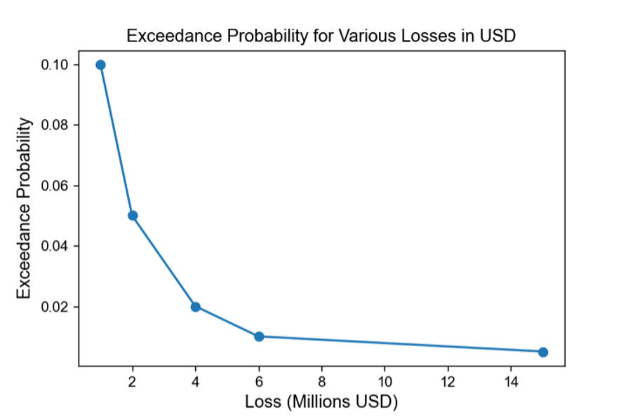
Figure 1: An example of an exceedance probability curve in catastrophe modeling. Each filled circle corresponds to the probability that a given loss will be exceeded in a time period.
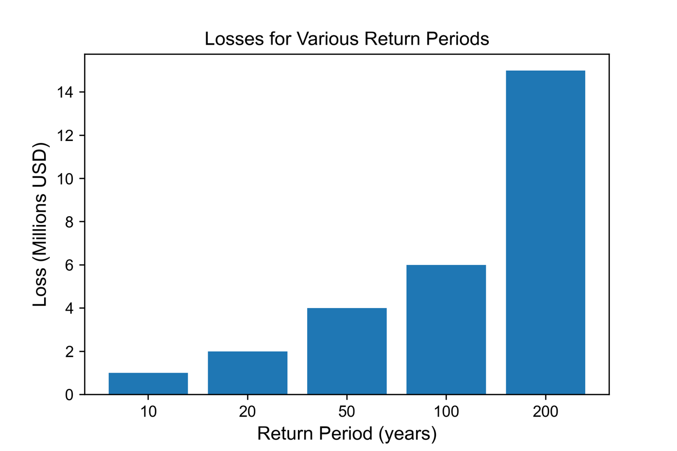
Figure 2: Exceedance probabilities in Figure 1 expressed in terms of return period (in years). Each bar on the graph represents the return period value for a given loss, which is the amount of time expected to pass for the recurrence of that loss.
Exceedance probabilities, or return periods, also can be used to characterize the hazard intensity one might experience over some period of time. For example, Kinetic Analysis has produced detailed maps of tropical cyclone wind speeds and storm surge for a variety of return periods. An example of return period maps for the Atlantic and Southwest Indian Ocean (SWIO) based on best-track data are shown in Figure 3. The plots represent wind speeds expected with a return period of 25 years based on events going back to 1950 for the Atlantic and Eastern Pacific and back to 1980 for other basins that experience tropical cyclones. The intensities are noisier for the SWIO region because the number of years of data and events are less than that for the Atlantic. The amount of smoothing can be adjusted if there is a need. An equivalent figure based on a stochastic catalog with 10,000 years of events for the Southwest Indian Ocean is shown in Figure 4. Note the figure is much smoother due to the greater number of events in the stochastic compared to the historical set.

Figure 3: Maps of 25-year return period wind speeds (using historical tropical cyclones) in two regions: (top) the Gulf of Mexico and western Atlantic and (bottom) the southwest Indian Ocean and southeastern coastline of Africa. The 25-year return period wind speeds shown in the top figure are based on the National Hurricane Center's best-track data for tropical cyclones that occurred from 1950 through 2021. The winds shown in the bottom figure are based on the Joint Typhoon Warning Center's best-track data for tropical cyclones that occurred from 1980 through 2021. The winds represent terrain-adjusted, 1-minute sustained winds at 10-meter elevation. Note that winds equal to or faster than the return period winds can occur more than once in a year, or in consecutive years.

Figure 4: Maps of 25-year return period wind speeds (using a 10,000-year stochastic set of tropical cyclones) in the southwest Indian Ocean and southeastern coastline of Africa. The winds represent terrain-adjusted, 1-minute sustained winds at 10-meter elevation. Note that winds equal to or faster than the return period winds can occur more than once in a year, or in consecutive years.
Another vital aspect of any catastrophe model is model validation [3]. Each component of the model must be carefully validated against data obtained from historical events [3]. The final output of the model is expected to be consistent with basic physical principles of the underlying hazard and unbiased when tested against both historical and real-time data [1, 3]. As we have discussed in this blog post, catastrophe models are complex yet elegant tools with many components. In part 2, we will discuss some of the common use cases of catastrophe models and how they have been employed across various industries.
References
1. https://www.air-worldwide.com/SiteAssets/Publications/Brochures/documents/about-catastrophe-models
2. https://www.rms.com/catastrophe-modeling?contact-us=cat-modeling#:~:text=Catastrophe%20modeling%20allows%20insurers%20and,hurricanes%20to%20floods%20and%20wildfires.
3. https://journals.ametsoc.org/view/journals/bams/85/11/bams-85-11-1713.xml
4. https://www.partnerre.com/wp-content/uploads/2017/08/catfocus-tropical-cyclone-model.pdf
5. https://www.casact.org/sites/default/files/2021-03/02_humphreys.pdf
6. https://www.mdpi.com/2073-4441/15/1/44#:~:text=The%20return%20period%20is%20the,6%2C7%2C8%5D.